Working In Uncertainty

Efficient samples for internal control and audit testing: Simple Bayesian formulae for Excel that reduce sample sizes

by Matthew Leitch; first appeared on www.irmi.com in January 2008

Two philosophies

There are, broadly, two ways of looking at evidence from samples and they derive from two very different traditions in statistics that have been battling it out for more than a century. Both have their advantages and disadvantages, their supporters and their detractors.

The most common one in auditing is based on the idea of estimating frequencies using assumed statistical distributions. The thinking is based on answering a question like this:

‘Assuming the actual error rate is a particular number, X, and that the errors are randomly distributed through the population of items to be audited, how many items would we have to test and find error free to be Y% confident that the actual error rate is no worse than some other number, Z?’

This works, provided that the actual error rate really is X, the errors are randomly distributed, and that you are lucky enough to find no errors in the sample. Otherwise it's back to the drawing board. You also have to make decisions about what Y and Z are, and pluck X out of the air. All these are difficult decisions because when you take them you know so little. There is an inherent circularity in finding an error rate by assuming an error rate at the start.

The less common approach to samples in auditing (though not in some other fields) is based on Bayes's rule and I think it is easier to follow. You start by being explicit about what you already know about the actual error rate, expressing it as a distribution over the whole range from 0 per cent error to 100 per cent error.

The distribution can be shown as a graph and what the graph looks like depends on what you already know about the error rate. Maybe you already suspect it is low, as shown in Figure 1, or perhaps you know nothing and so prefer to assume all error rates are equally likely, as in Figure 2.

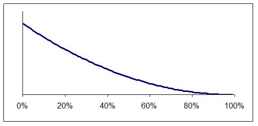
Figure 1: Low error rates seem more likely

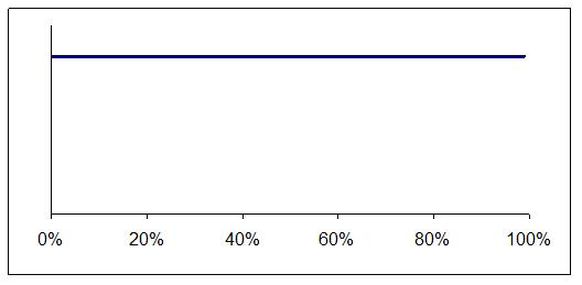
Figure 2: All error rates seem equally likely

As before, you (usually) assume that errors are randomly distributed. Then you sample one item and update your view of the likely error rate using the evidence from it. If the item was without error then your distribution nudges over to give more weight to lower error rates. One the other hand, if the item is in error then your distribution swings the other way, towards higher error rates.

For example, let's assume you started out thinking all error rates were equally likely. The first item you sample is without error. This alone proves very little but it does shift your view from Figure 2 to Figure 3.

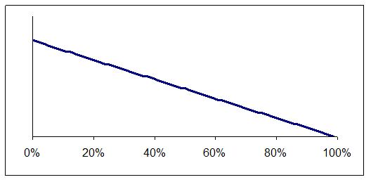
Figure 3: One item tested and found to be correct

As you sample each additional item you update your views each time. You can also test them in batches, but it makes no difference to the end result.

Eventually the evidence causes your distribution to get narrower and narrower, marking out the error rate with greater and greater tightness and certainty. For example, suppose you started with Figure 2 and then tested 100 items and found 3 errors. The result would be Figure 4.

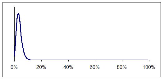
Figure 4: Three errors in 100 items tested

If you want to you can specify a stopping point, such as being Y per cent sure the error rate is no higher than Z. However, as you go along you can look at it in different ways, and show people the whole distribution so they can make up their own minds. Perhaps people were hoping the error rate could be shown to be below 2 per cent but results so far suggest it is probably in the 3 – 10 per cent range. It's time to think again and being able to see the whole distribution helps people understand the situation.

Spreadsheet formulae

For error rates in streams of transactions there is a very simple type of mathematical curve that can represent our views about the error rate and it is exceptionally simple to calculate how it changes as sample items are tested.

The curve is called a Beta distribution and is conveniently built into Microsoft Excel as BETADIST( ). It is also in other commonly used software.

BETADIST( ) gives you the probability that the error rate is below a given level for given values of two parameters that are set by your sample results.

For example, BETADIST(0.05, 3+1, 97+1) gives you the probability that the actual error rate is less than 5 per cent once you have tested 100 and found three errors. It's just under 75 per cent.

To create graphs such as the ones above you need to use BETADIST lots of times to convert the cumulative probabilities given by this function into approximate probability densities. For example, to find the data point at an error rate of 5 per cent you could use:

(BETADIST(0.05, 4, 98) – BETADIST(0.049, 4, 98) ) / 0.001.

The formulae given above assume you started out thinking all error rates were equally likely. If this was not your initial view then the technique is to act almost as if you have already tested a sample, starting from the ‘all equally likely’ assumption.

For example, Figure 1, above, was a curve for initial views that was equivalent to having tested two items and found them both to be correct. If that was our starting point then the probability of the error rate being below 5 per cent after testing 100 items and finding three errors would be BETADIST( 0.05, 3+1, 2+97+1), which is just over 76 per cent. It's slightly more than before because we started with a weak belief that the error rate was more likely to be low than high.

Cutting sample sizes

Using this Bayesian approach there are two ways to cut sample sizes.

The least important is to take advantage of information about error rates acquired before the sample test takes place. Perhaps you have information from sample tests in previous periods, or from some other type of test such as an overall analytical comparison. Or perhaps it is simply that you would be out of business if the error rate was anything other than small.

If any of these are true and you can justify starting with a distribution more like Figure 1 than Figure 2, or perhaps even tighter, then it will take fewer sample items to reach any given level of confidence about error rates.

Unfortunately, where very low error rates are involved (as is often the case in practice), this turns out to be a handful of sample items saved out of thousands. Do check in case your situation is different for some reason, but don't be optimistic.

The big opportunity to cut sample sizes comes from avoiding wasted sample items. The logic of the usual approach is to guess an error rate then work out a sample size that will deliver the target confidence. What if the actual error rate is higher? In this case you normally end up doing additional sample items. What if the actual error rate is lower? In this case you normally end up doing the number of items originally planned, even though that is more than you really need.

As you can see, whenever the actual error rate is lower than the rate you assumed to calculate the sample size you will end up doing unnecessary sample items.

Using the Bayes rule approach and continuously updating the analysis as each result comes in it is possible to stop work the moment the required confidence is reached. This is because the distribution represents all your beliefs about the true error rate, even taking into account what you believe you might find from additional testing.

On average, the number of sample items you test will be lower. Simple simulations can establish exactly how much lower in any given situation, and they can be used to test rules of thumb for extending samples in batches if that is more efficient.

Conclusion

The logic and calculations required for the Bayes rule approach are surprisingly simple and intuitive. I find the way the graphs change as data comes in mesmerizing, almost beautiful. It's also a practical approach. In a demonstration for a major telecoms company I showed that they could expect to cut average sample sizes by over 25% just by avoiding wasted sample items, despite some awkward industry regulations.